Simulation of custom binding systems

Return to tutorials

Example code for a simple binding system is available here: https://github.com/stevenshave/pybindingcurve/blob/master/example_custom_binding_system.py

A more complex example is also available here: https://github.com/stevenshave/pybindingcurve/blob/master/example_custom_binding_system2.py

PyBindingCurve is able to write custom functions representing a binding system from very simple system definition strings. This allows the simple definition, solving, plotting and fitting to any custom system.

We define these custom systems as simple strings with reactions separated either on newlines, commas, or a combination of the two. Reactions take the form:

• r1+r2<->p

Denoting that reactant1 + reactant2 bind together to make the product.

PBC will generate equations representing the custom system and use root finding techniques to calculate species concentrations at equilibrium. Readouts are signified by inclusion of a star (*) on a species. If no star is found, then the first seen product is used. Some system examples follow:

• “P+L<->PL” - standard protein-ligand binding
• “P+L<->PL, P+I<->PI” - competition binding
• “P+P<->PP” - dimer formation (default readout on PP - dimer)
• “P*+P<->PP” - dimer formation (readout specified on P - monomer)
• “monomer+monomer<->dimer” - dimer formation (default readout on PP)
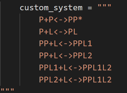
• “P+L<->PL1, P+L<->PL2, PL1+L<->PL1L2, PL2+L<->PL1L2” - 1:2 site binding

KDs passed to custom systems use underscores to separate species. P+L<->PL would require the KD passed as kd_p_l_pl. Running with incomplete system parameters will prompt for the correct ones. All species and KDs are cast to lower-case, simplifying parameter passing.

We can choose to work in a common unit, typically nM, or µM, as long as all numbers are in the same unit, the result is valid. We assume µM for all concentrations and KDs bellow.

To simulate a highly complex system, where protein binds to ligand, but protein can dimerize, while protein dimer binds to an inhibitor, and the protein dimer has can bind a single ligand, and our readout is on the protein monomer bound to ligand, we would define the system as follows:

custom_system="""
       P+L<->PL*
        P+P<->PP
        PP+I<->PPI
        PPI+L<->PPIL
"""

We can simulate this system in Python as follows:

import numpy as np
import pybindingcurve as pbc
custom_system="""
        P+L<->PL*
        P+P<->PP
        PP+I<->PPI
        PPI+L<->PPIL
"""
my_system = pbc.BindingCurve(custom_system)

We then define the system parameters in a python dictionary.

system_parameters = {
        'p': np.linspace(0,5), 
        'l':0.5,
        'i':4.0,
        'kd_p_l_pl':4.3,
        'kd_p_p_pp':1.2,
        'kd_pp_i_ppi':1.2,
        'kd_ppi_l_ppil':0.2,
}

We can now add the curve to the plot. If we want multiple simulations on the same plot, then it is good to give the curve a name with the optional name parameter.

my_system.add_curve(system_parameters, name= “Curve 1”)

Finally show the plot. Optionally, title, xlabel and ylabel variables may also be passed to title the plot and axes.

my_system.show_plot()

This produces the following plot:

To obtain exact single points from the plot, we may call the query function of my_system.

If a list or NumPy array is included as a system parameter, then a NumPy array of results is returned.

We may want to simulate a system in terms of a signal, not the concentration of complex. In this case, we may pass additional parameters, setting the ymax and/or ymin variables in the system parameters. Inclusion of these will scale the signal present between these values. This is very important if a detector is used with a maximum or minimum sensitivity and you wish to simulate response.

Return to tutorials