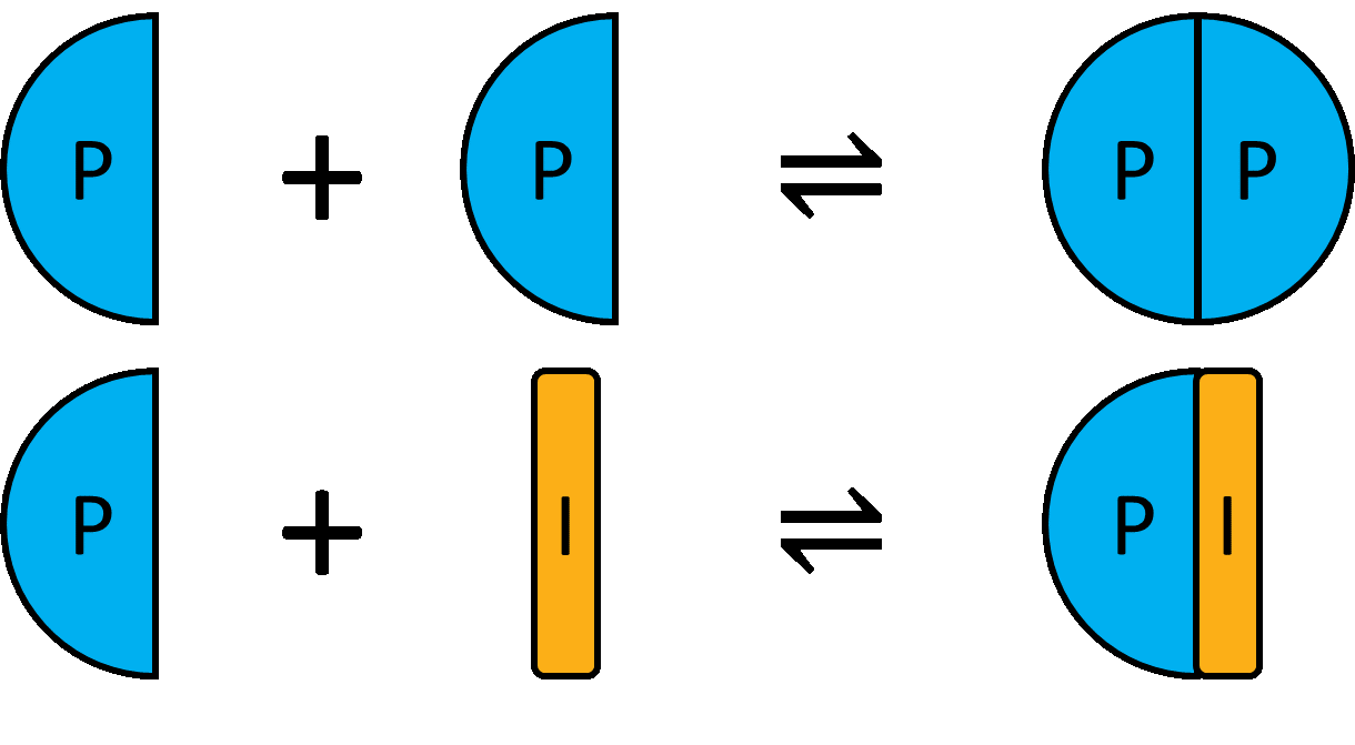
Fitting of data to homodimer formation

Return to tutorials

Using experimental competition data, we may obtain system parameters, such as dimerisation KD. Example code is available here: https://github.com/stevenshave/pybindingcurve/blob/master/example_homodimer_formation_fit.py Perform the standard imports:

import numpy as np
import pybindingcurve as pbc

We can choose to work in a common unit, typically nM, or µM, as long as all numbers are in the same unit, the result is valid. We assume µM for all concentrations bellow:

Define experimental data:

xcoords = np.array([0.0, 16.7, 33.3, 50.0, 66.7, 83.3, 100.0])
ycoords = np.array([0.0, 0.004, 0.021, 0.094, 0.312, 1.188, 3.854])

Construct the PyBindingCurve object, operating on a homodimer breaking system and add experimental data to the plot:

my_system = pbc.BindingCurve("homodimerbreaking")
my_system.add_scatter(xcoords, ycoords)

Known system parameters, kdpl will be added to this by fitting:

system_parameters = {"p": xcoords, "i": 100, "kdpp": 10}

Now we call fit, passing the known parameters, followed by a dict of parameters to be fitted along with an initial guess, pass the ycoords, and what the readout (ycoords) is:

fitted_system, fit_accuracy = my_system.fit(system_parameters, {"kdpi": 0}, ycoords)

Print out the fitted parameters:

for k, v in fit_accuracy.items():
    print(f"Fit: {k}={fitted_system[k]} +/- {v}")

Assign more points to ‘p’ to make a smooth plot:

fitted_system["p"] = np.linspace(0, np.max(xcoords))

Add a new curve, simulated using fitted parameters to our BindingCurve object and display the plot:

my_system.add_curve(fitted_system)
my_system.show_plot()

Resulting in:

Fit: kdpi=1.0024780308947485 +/- 0.001698935583536732

Return to tutorials